(Unpublished; adapted from the lecture presented at the Symposium on Music and the Cognitive Sciences, IRCAM, Paris, March 23 1991, organized by S. McAdams.)
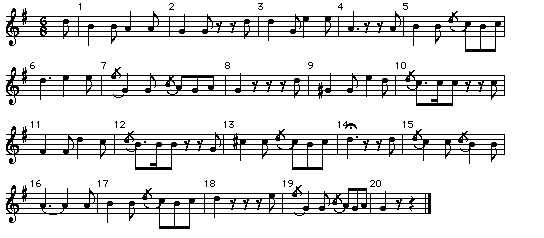
It is well known that in music performance an interpreter adds much information to the score. We will concentrate in this lecture on the timing aspects: if music is played, some of the required timing, tempo and changes thereof are explicitly notated in the score in the form of a global tempo marking or an accelerando or rallentando sign. But many more, and more subtle variations are performed either based on the structural features marked in the score (like bar lines or beaming of notes), or the interpretation of the piece by the performer. As an example for this lecture we will use the theme from the six variations composed by Beethoven over the duet Nel cor piò non mi sento.
The melody of theme from the six variations composed by Beethoven over the duet Nel cor piò non mi sento. The first example is a ridiculously metronomical performance made by computer of the theme from these six variations, in which all timing is solely derived from the explicit markings in the score (namely the note durations and the global tempo). All dynamic (loudness) information is ignored as is of course obligatory on a harpsichord, the instrument that we will simulate with the synthesizer. We will omit the accompaniment in all our examples, and concentrate only on the melody of the theme and its timing aspects.
![]()
All the grace notes are notated the same in the score, and also performed (by the computer) with the same duration. Though some of you might have judged some of them correct, other too short (The ones in bar 5, 12, 15 sound reasonable, the ones in bar 7 and 19 sound too short) But they are all played with the same duration. Now listen to the next example. What is different here?
![]()
We added some random timing of every note in the range from 0-10% of the tempo. A listeners creates structures (groupings) in this noise. Its sounds better than the metrical version. The next example is a real performance to show how much extra timing information is added to the score by a performer:
![]()
The first transformation we will try out is changing the key from G Major to G Minor, a feature that is built into any commercial sequencer nowadays. We will keep the original performed timing invariant. The following sound example is the result when applying this tempo pattern, found in a real performance to the almost the same material with only some pitches changed because of the change of mode:
![]()
But if we ask a human performer to play the piece in the minor key it sounds like:
![]()
Some might hear a clear difference here, others might have some difficulty.
Let's zoom into some detail to find out. For instance (the first fragment is the performed in minor, the second transformed major performance):
![]()
And another fragment from the same performance (again, the first fragment is the performed in minor, the second transformed major performance):
![]()
One might argue that a change of mode is not a minor change at all. It thoroughly upsets the structure of the piece. If this is true, one might want to look at another change that does not interfere with melodic or harmonic structure: a change of global tempo.
Once again, this is easy to accomplish on any sequencer program: they all have a tempo knob that can be freely adjusted. Let us listen to a speeded-up version of the original performance with a factor of 1.5 (from about tempo 60 to tempo 90):
![]()
This again sounds weird. The rubato is too much and abruptly. Some notes have a strange timing (e.g. the e in bar 4). Also some of the grace notes are performed wrong to some people taste. Lets check it with the performance of a human interpreter at the same high tempo (tempo 90):
![]()
What happened? The sequencer speeded everything up by the same amount whereas, in the performance, the expressive timing profile is not just played faster. The rubato is adapted according to the tempo. At the higher tempo the rubato is less deep. If a piece is played at another tempo, other structural levels become more important, for instance, at a higher tempo the tactus will shift to a higher level (of the metrical structure), the fine subdivisions of the beat will get more "out of focus", and the phrasing of longer time spans will gain in detail.
Even more noticeable are the local effects. For some notes the duration has not changed at all in the faster performance. Some of these notes are grace notes. They do not change at all when performed at an another tempo. But not all grace notes behave like this.
For example, the two grace notes that cover an interval of a sixth, in bar 7 and 19, are timed like any other note: they are actually played in a metrical way. Thus there are grace notes in the score that are notated in the same way, but that need a different interpretation. There is a difference between ornaments that either "crush in" notes (that are really ornaments that take up very little or no time) or "lean on" notes (ornaments that have an important melodic or harmonic function).
Lets pick out again some fragment to listen to them more closely. You will here the same fragment in three versions:
![]()
In this first example hardly any difference is noticeable. The grace notes apparently behave metrical, and can be scaled like the other notes.
![]()
In this example there is some difference. The grace note is to short is the scaled fragment. There seems to be a lower limit to the duration of the grace note (the first two grace notes are about 50 ms -they are both performances-, the latter is 1.5 times as short, around 30 ms Çthis is the scaled version).
![]()
The last example shows the freedom the pianist took in playing both grace notes (they are played very differently). Though, in the performed high tempo they both become the same short 'crushing-in' grace notes. The scaled version, of course, still has the same differentiation between the two grace notes. The fact that a simple sequencer program, that makes use of this tempo curve notion, cannot play the onsets of such ornaments correctly might be forgivable, but there are still more problems. It also cannot deal with the articulation of notes. The proportion of the notes' duration that is actually sounding seem to be played to short (they also cannot just be scaled to a higher tempo).
So, sequencers equipped with tempo knobs and tempo tracks are not so wonderful after all. They cannot be used to change something, because detailed knowledge about structural levels, articulation, and timing of ornamentation's, is indispensable. How dumb of us, after all, to assume that a tempo knob on a commercial sequencer package could be used to adjust the tempo.
As a preliminary conclusion, I will end with the observation that expressive timing seems to be so intimately linked to structure, that tempo curves, which totally ignore that fact, are only useful as a measurement device, and simple transformations are doomed to fail.
There are 3 well-known models that claim to generate expressive timing from a structural description of the music. I will explain them and let you hear how well they perform on our Beethoven piece.
By the way, all these sound examples were made with POCO, a kind of computer workbench for expressive timing. This system was developed in the past few years when we worked at City University in London together with Eric Clarke.
Let us start with Manfred Clynes' model, the so called composers' pulse. Clynes proposes composer specific and meter specific, discrete tempo patterns linked to a few levels of metrical structure. This composers' pulse is assumed to communicate the individual composers' personality. Clynes is opposed to analysis of performance data: the pulses stem from his own intuition. He even states that if a performer does not play a piece conforming to the rules of the composers pulse, then he or she does not understand the composers' personality well enough. For the Beethoven 6/8 pulse Clynes proposes to allot 49% of the duration of a bar to the first half bar and the remaining 51% of the bar duration to the second half bar. This procedure of unequal allotment is repeated for each half bar which is divided in 35, 29 and 36% for each subsequent beat. This model gives rise to the following tempo curve with repeating sections for each bar.
Let's listen first to the pulse in isolation. In the beginning the first beat of a bar and the fourth beat of a bar are indicated with different tones.
![]()
If we map this pulse to the Beethoven theme we get the following result:
![]()
So in this model all expressive timing stems from the metrical units half bar and beat - which of course is not enough. In systematic research as was done by Bruno Repp it appears that for some rhythmical material the composers pulse performs remarkably well, whereas for other material it is not so good. And in general meter explains the timing deviations found in musical performance to a limited extend, especially in the romantic period, when the large rubato patterns seem to communicate the phrase structure. That is the idea that Neil Todd elaborated. He states that the tempo in each phrase follows the following pattern: speeding up through the middle of the phrase, and slowing down at the end. The last phenomenon has its own name: phrase final lengthening. The form of these tempo changes can be formalized by describing the beat length by a so-called parabola curve. He then proposes that this process takes place at each level in a nested hierarchy of phrases and sub phrases. The results at each level combine to yield the tempo for the whole piece. And, indeed, if one looks at the tempo of the performed piece, it appears that the characteristic curves can be recognized, corresponding to a phrase structure analysis of the piece.
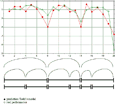
In this sheet the phrase structure indicated by our performers is shown, but other interpretations are possible. Each phrase and sub-phrase contributes its own curve. The combination of which is shown here, as is the real performance (with black dots). Now let us listen to this model.
![]()
Most notable in phrase final lengthening is the interaction with the actual rhythmical material. If a rubato is very heavy (like in bar 7) it may come close to altering the rhythm itself. Todd does not specify a method to yield appropriate parameter values for the curves, they have to be fitted to a real performance, and predictions about for instance the adaptation of the curves to global tempo is not explained. And of course it is again only a partial model, all structure other than phrase structure is ignored (the model specifies the phrase timing until beat-level).
It is noteworthy that a formalized generative model of the link between rhythmical grouping structure and expressive timing does not exist. There is some evidence for a systematic way in which certain rhythmical patterns are played: like a triplet in the context of a duple meter. But a general theory is still lacking, which seems a bit strange in the light of some recent evidence that rhythmic structure is responsible for a large proportion of the timing variance. The final generative model that I will explain ignores hierarchical structural descriptions and concentrates on the so called surface structure of the music: local features and patterns found in the note by note description of the score. Johan Sundberg proposes a rule system to generate expression from a score based on this surface structure. His research was done in a analysis-by-synthesis paradigm and captures expert intuition in the form of a large set of rules. A example of a rule is "Faster uphill": a duration of a note is shortened in performance if it is preceded by a lower pitched note and followed by a higher pitched one. There is a large set of these rules available (ca. 25) and the set is still growing . Some rules are applicable in our case. In the following sound example the rule, called ÑLeap tone durationæ was used. This rule changes the duration of two succeeding notes, adding time to the first and subtracting time from the second note, proportional to the size of the interval: the larger the interval leap the more the durations are distorted. This is quite noticeable in the following sections:
![]()
It turns out that the use of one or two rules is quite effective, but larger rule-cocktails are hard to judge. This is because it is unclear how rules interact and which classes of rules are dependent. So mixing them together gives unpredictable results. Furthermore, the effectiveness of a rule depends heavily on the material, the piece it is applied too (Sundberg uses in his articles another musical example for every rule).
As a conclusion about these three generative models one can say that they indeed model part of the link from structure to expression, but it is not at all clear how these incompatible structural descriptions yield a combined expressive timing profile. In the hope to find more results in the music itself we turn again to the measurement of performance data. One can question if such physical measurements of tempo or relative duration make any psychological sense. Do we perceive a duration that is 1.5 times as long indeed as 1.5 times as long? There has been done a lot of research on the subjective scales of time and tempo magnitude. Most psychophysical scales for time intervals are described by Stevens' Law, a power law that relates the physical magnitude of a stimulus with its perceived magnitude. For time duration the exponent is commonly found to be 1.1, a slight overestimation of the interval. However, for intervals shorter than 500 ms it is found that it is around 0.5, the subjective magnitude is the square root of the physical duration. But this research has all been done with impoverished stimulus material, often consisting of one or two time intervals marked-off with clicks. Other research found that duration judgment depends on the way the interval is filled with more or less events, so unfortunately these simple laws cannot be directly applied to more complex material like real music.
Now let us look at the way most authors present timing patterns. A
typical example is: 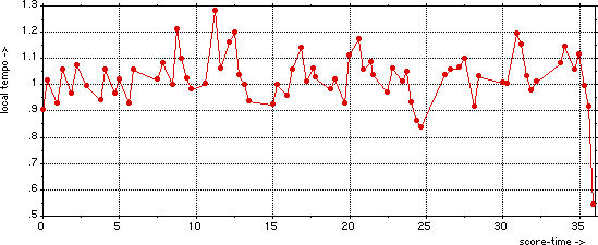
On the horizontal axis, score time is represented, on the vertical axis local tempo or velocity. One can see that this author connects the measurement points by a straight line. And, indeed, most timing or tempo measurements are presented in the form of a continuous curve instead of just a scattergram of measurements. These curves more or less imply an independent existence, apart from the rhythmic material from which they were measured. But one cannot perceive timing or tempo without events carrying it. The psychologist James Gibson even wrote an article called "Events are perceivable but time is not". And vise versa: "filling up" a time interval by adding an event between two measured points is problematic because it will change the perceived duration of the original interval.
But let's do a critical test and listen to the consequences of
representing tempo curves as an abstract entity. If it has indeed an
existence of its own we can detach it from the rhythmic material and
map it to another piece. The obvious piece to use here is of course
one of the variations. 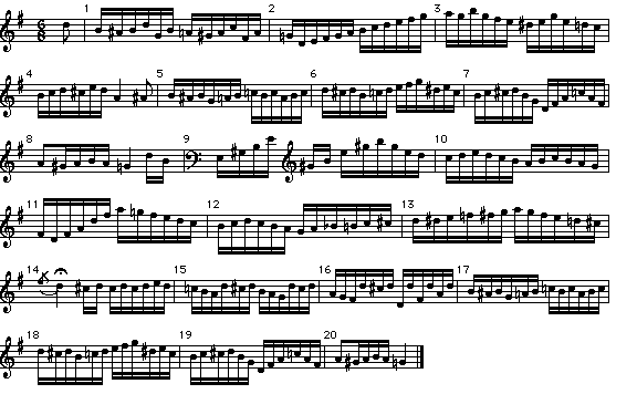
Let us first listen to the score of this first variation, performed mechanically, without expressive timing.
![]()
Now we can apply the tempo curve of the performance of the theme to this score of the variation. This is the result:
![]()
Most noticeable are the rushing passages in bar 7 and 9, due to the high local tempo found in the theme at those positions, but now used for more notes. A real performance of the variation sounds like this:
![]()
It is of course possible to do it the other way around: perform the theme with the tempo measured in the performance.
![]()
Here it is clear that e.g. the ritardandi start too early (like in bar 13). The examples show that a tempo curve indeed is so intimately linked to the material, that even a mapping to a piece that is very much related, cannot be done.
The Figure above shows how the actual mapping was done. First, we have tempo measurements at each note in the theme and we need to invent the tempo of notes that are added in the variation. One way is to assume that the tempo stays constant during that period, That is the mapping you just heard. But of course it sounds a bit 'jumpy'. If we follow the authors that draw tempo curves of straight line segments, we would get this kind of linear interpolation. At Ircam, David Wessel and colleagues worked at even smoother interpolations of tempo curves, using so called splines.
Now listen to the result of such a smoothing of the tempo curve measured in a performance of the theme and applied to the variation:
![]()
This indeed is a smooth way of using rubato and it sounds better than the previous example, but it is still far from a real performance, because again it lacks the link to the structural details of the variation.
Now we come to the conclusion. We hope to have shown that we must be aware of the Tempo Curve. Of course, one should be encouraged to measure tempo curves and use them for the study of expressive timing. But it is a dangerous notion, despite its widespread use, because it lulls its users into the false impression that it has a musical and psychological reality. There is no abstract tempo curve in the music nor is there a mental tempo curve in the head of a performer or listener. And any transformation or manipulation based on the implied characteristics of such a notion is doomed to fail. That does not mean that generic models that represent timing in terms of some sort of structure, even when they describe just a fraction of the many aspects of expressive timing, do constitute a valuable contribution to the field. They only have to be seen in a proper perspective in which their limitations are understood as well. It also does not mean that certain features in computer music software and commercial sequencers, like a tempo knob, should be forbidden. Their mere existence at least makes the realization of their limited worth evident.